Identifying Frequent Stops with GTFS
- Counting by Route
- Counting by Stops
- Measuring Frequency Much More Precisely
- Analysis with GraphViz
- The Final Result
- Bonus: Utility Views
Sometimes when I’m doing analysis I find myself needing to figure out how many services each route (or stop/station) has in a week, or if a location has frequent service.
In writing this article, it became apparent that I use the term
“service” in a few different ways - in the generic sense of “Sunday
service”, which is close to a GTFS Service - to refer to a
specific instance of a route (which GTFS refers to as
Trip): a vehicle starts at a stop, it terminates at a stop,
and it visits some number of stops in between.
It’s the latter type of services that we’re counting.
Please note: I went through a heap of different ideas along the way here. Jump right down to Measuring Frequency Much More Precisely for the best version.
We’ll use (static) GTFS data for TransLink SEQ.
Counting by Route
First, here’s a way to count by routes. It’s what initially occurred to me — but it’s also fatally flawed.
SELECT count(*) as incorrect_count, route_short_name, direction_id
FROM StopTimes JOIN Trips USING (trip_id) JOIN Routes using (route_id)
WHERE stop_sequence = 1
GROUP BY route_short_name, direction_id
-- limit 3
;
After most samples of SQL code I’ll present a table with just a few of the results. Sometimes they’ll be manually selected, but often the criteria will be commented out in the code.
| incorrect_count | route_short_name | direction_id |
|---|---|---|
| 782 | 100 | 0 |
| 792 | 100 | 1 |
| 102 | 101 | 0 |
Note: GTFS files are effectively CSVs. Since this is relational data,
I like to import them into SQLite (everything is text, but we can deal
with that). I also name the resulting tables such that, for example,
stop_times.txt becomes StopTimes.
CREATE TABLE IF NOT EXISTS "Routes" (
"route_id" TEXT, "route_short_name" TEXT, "route_long_name" TEXT, "route_desc" TEXT,
 "route_type" TEXT, "route_url" TEXT, "route_color" TEXT, "route_text_color" TEXT);


CREATE TABLE IF NOT EXISTS "StopTimes" (
"trip_id" TEXT, "arrival_time" TEXT, "departure_time" TEXT, "stop_id" TEXT,
 "stop_sequence" TEXT, "pickup_type" TEXT, "drop_off_type" TEXT);
CREATE INDEX idx_stoptimes_trips ON StopTimes (trip_id);
What’s the issue with that first bit of code? Well,
StopTimes says when in the day a service runs, but
not which day, let alone date, it runs on. Weekdays, weekends,
public holidays, service changes — all in there together.
Let’s look at the Trips table:
CREATE TABLE IF NOT EXISTS "Trips" (
"route_id" TEXT, "service_id" TEXT, "trip_id" TEXT, "trip_headsign" TEXT,
 "direction_id" TEXT, "block_id" TEXT, "shape_id" TEXT);

CREATE UNIQUE INDEX pk_trips on Trips (trip_id);
What’s this service_id column? It only appears in two
other tables, namely Calendar and
CalendarDates. 1
This is actually how GTFS specifies which trips occur on a given
date! Calendar encodes normal operations (allowing for a
pattern which repeats every week) while CalendarDates
encodes exceptions on specific dates (like public holidays).2
CREATE TABLE IF NOT EXISTS "Calendar"(
"service_id" TEXT, "monday" TEXT, "tuesday" TEXT, "wednesday" TEXT,
 "thursday" TEXT, "friday" TEXT, "saturday" TEXT, "sunday" TEXT,
 "start_date" TEXT, "end_date" TEXT);

CREATE TABLE IF NOT EXISTS "CalendarDates"(
"service_id" TEXT, "date" TEXT, "exception_type" TEXT);

CREATE UNIQUE INDEX pk_calendar ON Calendar (service_id);
CREATE UNIQUE INDEX pk_calendar_dates ON CalendarDates (service_id, date);
Note that the dates in CalendarDates are single days and
override the day-of-the-week columns in Calendar.
For example, a particular service might be specified as
sunday-only service in Calendar, but apply
most days from Christmas Day to January 1st in
CalendarDates. As for exception_type, a
1 is an added service and a 2 is a removed
service.
Here’s some entries from Calendar:
| service_id | monday | tuesday | wednesday | thursday | friday | saturday | sunday | start_date | end_date |
|---|---|---|---|---|---|---|---|---|---|
| GCLR 24_25-36993 | 0 | 0 | 0 | 0 | 1 | 0 | 0 | 20250124 | 20250321 |
| GCLR 24_25-36991 | 1 | 1 | 1 | 1 | 0 | 0 | 0 | 20250123 | 20250324 |
| GCLR 24_25-36990 | 0 | 0 | 0 | 0 | 0 | 1 | 0 | 20250125 | 20250322 |
| GCLR 24_25-36992 | 0 | 0 | 0 | 0 | 0 | 0 | 1 | 20250126 | 20250323 |
| ATS_SBL 25-38504 | 0 | 0 | 0 | 0 | 0 | 1 | 0 | 20250315 | 20250315 |
And from CalendarDates:
| service_id | date | exception_type |
|---|---|---|
| BBL 24_25-36196 | 20250127 | 2 |
| BCC 24_25-38101 | 20250127 | 1 |
| CBL 24_25-36455 | 20250127 | 1 |
| ATS_TBS 25-38421 | 20250130 | 2 |
| ATS_TBS 25-38421 | 20250131 | 2 |
So to answer the question “How many trips run each week?” we need to:
- Choose a week (i.e. a start and end date). For each date in that
week:
- Identify all the services usually running during that day
(using
Calendar)- A service is usually running if
{date} BETWEEN start_date AND end_dateand if the day-of-the-week column is1 - Note that a service might start on, say, the Wednesday in the middle of our chosen week, but also define services running on Mondays and Tuesdays (presumably starting the following week). This is part of why we have to go day-by-day.
- A service is usually running if
- Identify any exceptions (using
CalendarDates) and apply those.- A service is included if its
exception_typeis1and excluded if it is2, for the relevant date. If it does not appear at all, only what’s inCalendarmatters
- A service is included if its
- Identify all the services usually running during that day
(using
- Then we can sum up by
service_id.
Notice that we don’t actually look at the StopTimes
table here at all!
Just for one day
Let’s begin by just calculating each day of the week separately, as
their own view. This is partly to avoid going full wizard upfront, and
partly because GTFS dates are in YYYYMMDD format rather
than YYYY-MM-DD.
-- Choose your own date (e.g. with parameter substitution)
-- Also do this for the other days of the week, swapping out the `monday` column
CREATE VIEW MondayServices AS
WITH
Inclusions AS
    (SELECT service_id FROM CalendarDates WHERE date = 20250203 AND exception_type = 1),
Exclusions AS
    (SELECT service_id FROM CalendarDates WHERE date = 20250203 AND exception_type = 2)
SELECT service_id FROM Calendar
WHERE (
    (start_date <= 20250203 AND end_date >= 20250203 AND monday = 1)
    AND (NOT (service_id in Exclusions)))
OR (service_id IN Inclusions);
The full week
Since there are only seven days in a week and our reference week might cross months, we can hard-code a common table expression like so, mapping dates to days of the week:
WITH
Dates (date, monday, tuesday, wednesday, thursday, friday, saturday, sunday)
AS (VALUES
   (20250203, 1,0,0,0,0,0,0),
   (20250204, 0,1,0,0,0,0,0),
   (20250205, 0,0,1,0,0,0,0),
   (20250206, 0,0,0,1,0,0,0),
   (20250207, 0,0,0,0,1,0,0),
   (20250208, 0,0,0,0,0,1,0),
   (20250209, 0,0,0,0,0,0,1)
)
-- rest of the query
Calling this from regular code, of course, we can use parameter
substitution. In SQLite that might look like this (assuming
$1 as the syntax for a substituted parameter). We can also
use date arithmetic to just pass the Monday (expected input format:
YYYY-MM-DD, with the dashes):
WITH
Dates (date, monday, tuesday, wednesday, thursday, friday, saturday, sunday)
AS (VALUES
   (strftime('%Y%m%d', date($1, '+0 day')), 1,0,0,0,0,0,0),
   (strftime('%Y%m%d', date($1, '+1 day')), 0,1,0,0,0,0,0),
   (strftime('%Y%m%d', date($1, '+2 day')), 0,0,1,0,0,0,0),
   (strftime('%Y%m%d', date($1, '+3 day')), 0,0,0,1,0,0,0),
   (strftime('%Y%m%d', date($1, '+4 day')), 0,0,0,0,1,0,0),
   (strftime('%Y%m%d', date($1, '+5 day')), 0,0,0,0,0,1,0),
   (strftime('%Y%m%d', date($1, '+6 day')), 0,0,0,0,0,0,1)
)
-- rest of the query
We will have to LEFT JOIN to CalendarDates
and rewrite Inclusions and Exclusions as
subqueries, as those CTEs assumed a specific date.
We match an entry from CalendarDates if any day
from our Dates table matches (and is active). Thankfully,
SQLite is very flexible and lets us do Boolean logic on text.
WITH
Dates (date, monday, tuesday, wednesday, thursday, friday, saturday, sunday)
AS (VALUES
   (20250203, 1,0,0,0,0,0,0),
   (20250204, 0,1,0,0,0,0,0),
   (20250205, 0,0,1,0,0,0,0),
   (20250206, 0,0,0,1,0,0,0),
   (20250207, 0,0,0,0,1,0,0),
   (20250208, 0,0,0,0,0,1,0),
   (20250209, 0,0,0,0,0,0,1)
)
SELECT
date, service_id, exception_type
FROM Dates JOIN Calendar
    ON ((Dates.monday AND Calendar.monday)
        OR (Dates.tuesday AND Calendar.tuesday)
        OR (Dates.wednesday AND Calendar.wednesday)
        OR (Dates.thursday AND Calendar.thursday)
        OR (Dates.friday AND Calendar.friday)
        OR (Dates.saturday AND Calendar.saturday)
        OR (Dates.sunday AND Calendar.sunday)
        )
    LEFT JOIN CalendarDates USING (date, service_id)
WHERE
    ((start_date <= date AND end_date >= date)
        AND (exception_type is null OR exception_type <> 2))
    OR (exception_type = 1)
;
Update: on first publication I made an embarrassing error switching the values of exception_type in the above code block. Fixed now!
I’ve included exception_type in the outputs for
diagnostic purposes. A few rows:
| date | service_id | exception_type |
|---|---|---|
| 20250203 | GCLR 24_25-36991 | |
| 20250203 | BBL 24_25-36196 | |
| 20250203 | ATS_TBS 25-38421 | 2 |
| 20250204 | QR 24_25-38716 |
We also need to count the number of days in the reference week each
service occurs, which is just a standard COUNT(*) and
GROUP BY. Let’s encapsulate it all in a view for good
measure.
CREATE VIEW WeeklyServices AS
WITH
Dates (date, monday, tuesday, wednesday, thursday, friday, saturday, sunday)
AS (VALUES
   (20250203, 1,0,0,0,0,0,0),
   (20250204, 0,1,0,0,0,0,0),
   (20250205, 0,0,1,0,0,0,0),
   (20250206, 0,0,0,1,0,0,0),
   (20250207, 0,0,0,0,1,0,0),
   (20250208, 0,0,0,0,0,1,0),
   (20250209, 0,0,0,0,0,0,1)
)
SELECT
count(*) as day_count, service_id
FROM Dates JOIN Calendar
    ON ((Dates.monday AND Calendar.monday)
        OR (Dates.tuesday AND Calendar.tuesday)
        OR (Dates.wednesday AND Calendar.wednesday)
        OR (Dates.thursday AND Calendar.thursday)
        OR (Dates.friday AND Calendar.friday)
        OR (Dates.saturday AND Calendar.saturday)
        OR (Dates.sunday AND Calendar.sunday)
        )
    LEFT JOIN CalendarDates USING (date, service_id)
WHERE
    ((start_date <= date AND end_date >= date)
        AND (exception_type is null OR exception_type <> 2))
    OR (exception_type = 1)
GROUP BY service_id
ORDER BY service_id
;| day_count | service_id |
|---|---|
| 4 | GCLR 24_25-36991 |
| 5 | BBL 24_25-36196 |
| 5 | ATS_TBS 25-38421 |
| 3 | QR 24_25-38716 |
Putting it all together
Now that we have our WeeklyServices view we can put
everything together!
SELECT sum(day_count) as service_count, route_short_name, direction_id
FROM Trips JOIN Routes using (route_id) JOIN WeeklyServices using (service_id)
GROUP BY route_short_name, direction_id
;| service_count | route_short_name | direction_id |
|---|---|---|
| 532 | 100 | 0 |
| 539 | 100 | 1 |
| 380 | 29 | 0 |
| 926 | GCR1 | 0 |
| 913 | GCR1 | 1 |
In the above query I’ve disaggregated by direction_id since some services (like the 29) are scheduled as one-way loops. We can take the max or min over this to get an idea of overall service quality while allowing for this sort of loop.
SELECT MIN(service_count), route_short_name FROM (
    SELECT sum(day_count) as service_count, route_short_name, direction_id
    FROM Trips JOIN Routes using (route_id) JOIN WeeklyServices using (service_id)
    GROUP BY route_short_name, direction_id
) GROUP BY route_short_name
HAVING MIN(service_count) >= (7 * 12 * 4)
    -- average 4 services an hour, 12 hours a day, 7 days a week
;| MIN(service_count) | route_short_name |
|---|---|
| 532 | 100 |
| 380 | 29 |
| 913 | GCR1 |
Counting by Stops
Knowing the number of Trips each Route takes is nice,
but often we care about more geographically-oriented issues like “is
this stop served by a route (or combination thereof) which comes at
least X times each day?”.
We could just identify the stops served by each frequent route. But there’s an issue here: Any individual trip might only visit some of the stops on a route (conversely, on some routes a trip might visit the same stop multiple times).
We have a few common scenarios: - Extensions and variations: some trips visit some extra or different stops, usually towards one end of the route. - Expresses: some trips skip stops in the middle of the route. - Partial runs: a trip serves only a fraction of the stops along the route. - In Brisbane, the orbital Great Circle line is served this way; each trip usually only covers about 1/3rd of the full route and some very short trips provide a once-a-day variations. - Complex loops: figure-eights, triquetras, cloverleafs may result in some stops being visited multiple times per trip while most stops are visited only once. - While uncommon, the same trip might perform multiple effective laps of the route, serving every stop multiple times.
It’s difficult to resolve this other than on a route-by-route basis.
My fluvial tool aims to go much more in-depth on the
topic of merging multiple runs into a single ordering. To stay in
relatively straightforward SQL, we should potentially figure out a way
to normalise each trip by the fraction of stops on the route it
serves.
To do this we need to bring back the StopTimes table.
The following code counts the number of times each week each route
visits each stop:
SELECT sum(day_count) as service_count, route_short_name, direction_id, stop_id
FROM StopTimes JOIN Trips using (trip_id) JOIN Routes using (route_id) JOIN WeeklyServices using (service_id)
-- WHERE route_short_name = 598
GROUP BY route_short_name, direction_id, stop_id
;| service_count | route_short_name | direction_id | stop_id |
|---|---|---|---|
| 135 | 598 | 1 | 10306 |
| 136 | 598 | 1 | 10679 |
| 141 | 598 | 1 | 10926 |
We can often also expose how trips serve different parts of a route
by looking at Trips.shape_id if available:
SELECT sum(day_count) as service_count, route_short_name, direction_id, shape_id
FROM Trips JOIN Routes using (route_id) JOIN WeeklyServices using (service_id)
-- WHERE route_short_name = 598
GROUP BY route_short_name, direction_id, shape_id
;| service_count | route_short_name | direction_id | shape_id |
|---|---|---|---|
| 6 | 598 | 1 | 5980008 |
| 135 | 598 | 1 | 5980009 |
| 130 | 598 | 1 | 5980010 |
| 130 | 598 | 1 | 5980011 |
| 6 | 598 | 1 | 5980012 |
| 5 | 598 | 1 | 5980013 |
| 5 | 598 | 1 | 5980014 |
| 6 | 598 | 1 | 5980203 |
The 598 is an unusually weird route in that buses start service at several different locations around the loop, some only once a day!
Something we might want to do the most is take the average number of times a route visits each of its stops. If we’re interested in the frequent network, we’ll probably want to approximate membership by thresholding that average too.
SELECT round(avg(service_count)) as avg_services, route_short_name, direction_id
FROM (
    SELECT sum(day_count) as service_count, route_short_name, direction_id, stop_id
    FROM StopTimes JOIN Trips using (trip_id) JOIN Routes using (route_id) JOIN WeeklyServices using (service_id)
    WHERE stop_id = 300304
    GROUP BY route_short_name, direction_id, stop_id
)
GROUP BY route_short_name, direction_id
HAVING avg_services >= (7 * 12 * 4)
;| avg_services | route_short_name | direction_id |
|---|---|---|
| 433.0 | 704 | 1 |
Having thresholded the routes, we can join everything back up to get a list of stops:
CREATE VIEW FrequentIndividualStops AS
WITH AvgServices AS (
    SELECT round(avg(service_count)) as avg_services, route_short_name, direction_id
    FROM (
        SELECT sum(day_count) as service_count, route_short_name, direction_id, stop_id
        FROM StopTimes JOIN Trips using (trip_id) JOIN Routes using (route_id) JOIN WeeklyServices using (service_id)
        GROUP BY route_short_name, direction_id, stop_id
    )
    GROUP BY route_short_name, direction_id
    HAVING avg_services >= (7 * 12 * 4)
)
SELECT stop_id, stop_lat, stop_lon
FROM Stops
    JOIN StopTimes USING (stop_id)
    JOIN Trips using (trip_id)
    JOIN Routes using (route_id)
    JOIN AvgServices using (route_short_name, direction_id)
GROUP BY stop_id
;
Perhaps we know that on some corridors, individual routes are not frequent but their combination is. We can identify stops which approach frequent service even if their routes are not:
SELECT sum(day_count) as service_count, stop_id
FROM StopTimes JOIN Trips using (trip_id) JOIN WeeklyServices using (service_id)
-- where stop_id between '1797' and '1802'
GROUP BY stop_id
HAVING service_count >= (7 * 12 * 4)
;| service_count | stop_id |
|---|---|
| 631 | 1797 |
| 632 | 1802 |
The Stops table also allows for stops to be grouped via
the parent_station field. We should too. Note that by
default the sqlite3 CLI imports missing CSV values as empty
strings, not as null, hence the nullif wrapper
for parent_station.
SELECT sum(day_count) as service_count, coalesce(nullif(parent_station, ''), stop_id) as combo_id, direction_id, stop_lat, stop_lon
FROM StopTimes JOIN Trips using (trip_id) JOIN WeeklyServices using (service_id) JOIN Stops using (stop_id)
-- where combo_id like 'place_intuq'
GROUP BY combo_id, direction_id
HAVING service_count >= (7 * 12 * 4)
;| service_count | combo_id | direction_id | stop_lat | stop_lon |
|---|---|---|---|---|
| 861 | place_intuq | 0 | -27.497974 | 153.011139 |
| 1065 | place_intuq | 1 | -27.497798 | 153.011170 |
Stops which make it over the threshold are likely to also include interchanges of multiple non-frequent routes, and places which occur multiple times in a route. Since these aren’t necessarily “on the frequent network” there’s a need for manual review here.
Measuring Frequency Much More Precisely
Up until now, we’ve been using a simple
7 * 12 * 4 = 336 services/week approximation of frequency.
But what about when a combination of peak-hour services and
more-than-12-hour span push the number of services per day over our
threshold, while still leaving gaps in the middle of the day?
Ideally, we would measure headways throughout the day, or even look at effective frequency.
Doing this at scale will also allow us to take more advantage of the concept of corridors. If a pair of locations (stops or stations) are connected, bidirectionally, at sufficient frequency, then that is exactly the definition of a link in the frequent network, and moreover one which does not depend on individual routes being frequent. It’s possible that there are actually several, disconnected frequent networks.
We can identify all adjacent 3 pairs of stops linked by a trip:
CREATE VIEW AdjacentStops AS
SELECT trip_id, departure_time, stop_sequence, stop_id,
    lead(stop_id) OVER (partition by trip_id order by cast(stop_sequence as int) ASC) as next_stop_id
FROM StopTimes
;| trip_id | departure_time | stop_sequence | stop_id | next_stop_id |
|---|---|---|---|---|
| 28348512-BBL 24_25-36196 | 06:30:00 | 1 | 12105 | 313180 |
| 28348512-BBL 24_25-36196 | 06:39:00 | 2 | 313180 | 313177 |
| 28348512-BBL 24_25-36196 | 06:40:00 | 3 | 313177 | 316811 |
What we now need to do is:
- For each day we’re interested in
- For each pair of stops
- Identify the headways between trips serving that pair
- For each pair of stops
This then allows us to say if they’re connected adequately frequently.
The following SQL will tend to produce a lot of rows with
departure = next_departure. This is because there are lots
of different trips corresponding to different services, each of which
may or may not be operating on any given day. Instead, I’ve filtered to
show a low-frequency route with only one service pattern, so it’s easier
to make sense of the format.
SELECT stop_id, next_stop_id, departure_time,
    lead(departure_time) OVER (partition by stop_id, next_stop_id order by departure_time asc) as next_departure
FROM AdjacentStops
WHERE next_stop_id is not null
-- and stop_id in ('12105', '313180', '313177')
ORDER BY departure_time asc
;| stop_id | next_stop_id | departure_time | next_departure |
|---|---|---|---|
| 12105 | 313180 | 06:30:00 | 17:48:00 |
| 313180 | 313177 | 06:39:00 | 17:57:00 |
| 313177 | 316811 | 06:40:00 | 17:58:00 |
Let’s generalise over the full week:
WITH
Dates (date, monday, tuesday, wednesday, thursday, friday, saturday, sunday)
AS (VALUES
   (20250203, 1,0,0,0,0,0,0),
   (20250204, 0,1,0,0,0,0,0),
   (20250205, 0,0,1,0,0,0,0),
   (20250206, 0,0,0,1,0,0,0),
   (20250207, 0,0,0,0,1,0,0),
   (20250208, 0,0,0,0,0,1,0),
   (20250209, 0,0,0,0,0,0,1)
),
ThisWeek AS
( SELECT
    service_id, date
    FROM Dates JOIN Calendar
        ON ((Dates.monday AND Calendar.monday)
            OR (Dates.tuesday AND Calendar.tuesday)
            OR (Dates.wednesday AND Calendar.wednesday)
            OR (Dates.thursday AND Calendar.thursday)
            OR (Dates.friday AND Calendar.friday)
            OR (Dates.saturday AND Calendar.saturday)
            OR (Dates.sunday AND Calendar.sunday)
            )
        LEFT JOIN CalendarDates USING (date, service_id)
    WHERE
        ((start_date <= date AND end_date >= date)
            AND (exception_type is null OR exception_type <> 2))
        OR (exception_type = 1)
)
SELECT date, stop_id, next_stop_id, departure_time,
    lead(departure_time) OVER
        (partition by date, stop_id, next_stop_id order by departure_time asc)
        as next_departure
FROM AdjacentStops
    JOIN Trips USING (trip_id)
    JOIN ThisWeek using (service_id)
WHERE next_stop_id is not null
;
This takes a pretty long time to run, so I materialized it and
indexed by stop_id.
CREATE TABLE MV_StopStopFreqs(
  date,
  stop_id TEXT,
  next_stop_id,
  departure_time TEXT,
  next_departure
); -- AS SELECT * FROM ...
CREATE INDEX idx_mvssf_stopid on MV_StopStopFreqs (stop_id);
Combined Routes, Combined Locations
In addition to combining frequency across all routes between stops, we also want to use combined locations where they exist. It wouldn’t do to miss out on frequency just because Route 1 leaves from Platform A and Route 2 leaves from Platform B while both serve the same pair of stations!
It’s probably best to start back at AdjacentStops,
turning it into AdjacentLocations…
CREATE VIEW AdjacentLocations AS
SELECT trip_id, departure_time, stop_sequence,
    coalesce(nullif(X.parent_station, ''), A.stop_id) as this_loc,
    coalesce(nullif(Y.parent_station, ''), A.next_stop_id) as next_loc
FROM AdjacentStops A
    JOIN Stops X ON (A.stop_id = X.stop_id)
    JOIN Stops Y ON (A.next_stop_id = Y.stop_id)
;
Then materialize and index the big query…
CREATE TABLE MV_LocationPairFreqs AS
WITH
Dates (date, monday, tuesday, wednesday, thursday, friday, saturday, sunday)
AS (VALUES
   (20250203, 1,0,0,0,0,0,0),
   (20250204, 0,1,0,0,0,0,0),
   (20250205, 0,0,1,0,0,0,0),
   (20250206, 0,0,0,1,0,0,0),
   (20250207, 0,0,0,0,1,0,0),
   (20250208, 0,0,0,0,0,1,0),
   (20250209, 0,0,0,0,0,0,1)
),
ThisWeek AS
( SELECT
    service_id, date
    FROM Dates JOIN Calendar
        ON ((Dates.monday AND Calendar.monday)
            OR (Dates.tuesday AND Calendar.tuesday)
            OR (Dates.wednesday AND Calendar.wednesday)
            OR (Dates.thursday AND Calendar.thursday)
            OR (Dates.friday AND Calendar.friday)
            OR (Dates.saturday AND Calendar.saturday)
            OR (Dates.sunday AND Calendar.sunday)
            )
        LEFT JOIN CalendarDates USING (date, service_id)
    WHERE
        ((start_date <= date AND end_date >= date)
        AND (exception_type is null OR exception_type <> 2))
        OR (exception_type = 1)
)
SELECT date, this_loc, next_loc, departure_time,
    lead(departure_time) OVER
        (partition by date, this_loc, next_loc order by departure_time asc)
        as next_departure
FROM AdjacentLocations
    JOIN Trips USING (trip_id)
    JOIN ThisWeek using (service_id)
WHERE next_loc is not null
;


CREATE INDEX idx_lpf_this_loc ON MV_LocationPairFreqs (this_loc);

-- select * from MV_LocationPairFreqs where this_loc = '313177';| date | this_loc | next_loc | departure_time | next_departure |
|---|---|---|---|---|
| 20250203 | 313177 | 316811 | 06:40:00 | 17:58:00 |
| 20250203 | 313177 | 316811 | 17:58:00 | 18:40:00 |
| 20250203 | 313177 | 316811 | 18:40:00 | |
| 20250204 | 313177 | 316811 | 06:40:00 | 17:58:00 |
| 20250204 | 313177 | 316811 | 17:58:00 | 18:40:00 |
| 20250204 | 313177 | 316811 | 18:40:00 | |
| 20250205 | 313177 | 316811 | 06:40:00 | 17:58:00 |
| 20250205 | 313177 | 316811 | 17:58:00 | 18:40:00 |
| 20250205 | 313177 | 316811 | 18:40:00 | |
| 20250206 | 313177 | 316811 | 06:40:00 | 17:58:00 |
| 20250206 | 313177 | 316811 | 17:58:00 | 18:40:00 |
| 20250206 | 313177 | 316811 | 18:40:00 | |
| 20250207 | 313177 | 316811 | 06:40:00 | 17:58:00 |
| 20250207 | 313177 | 316811 | 17:58:00 | 18:40:00 |
| 20250207 | 313177 | 316811 | 18:40:00 |
Picking Winners
Remember, we want to know whether or not a given stop stop maintains decent frequency all day every day.
This SQL checks that the headway between subsequent services is 15 minutes or less, 7AM to 7PM, for the dates Monday 3rd through Friday 7th of February, 2025.
WITH Span AS (
    SELECT * FROM MV_LocationPairFreqs
    WHERE
        departure_time BETWEEN '07:00:00' AND '19:00:00'
        AND date BETWEEN 20250203 AND 20250207
),
Diffs AS (
SELECT this_loc, next_loc,
    max(timediff(next_departure, departure_time)) as maxdiff
FROM Span
GROUP BY this_loc, next_loc
HAVING maxdiff BETWEEN '+0000-00-00 00:00:00.001' AND '+0000-00-00 00:15:00.000'
),
FreqStopIds AS (
    SELECT this_loc as stop_id FROM Diffs
    UNION
    SELECT next_loc as stop_id FROM Diffs
)
SELECT stop_id, stop_name, stop_lat, stop_lon
FROM FreqStopIds JOIN Stops USING (stop_id)
-- limit 2
;| stop_id | stop_name | stop_lat | stop_lon |
|---|---|---|---|
| 10 | Ann Street Stop 10 at King George Square | -27.468003 | 153.023970 |
| 10079 | Mollison St near Melbourne St, stop 5 | -27.477055 | 153.011924 |
Now we can do useful things like mapping the frequent network!
I found that this included less stops than I expected, perhaps due to the occasional greater-than-15-minute headway.
In order to be robust and allow a few lapses, we should probably adopt a percentile-based approach or even an effective-frequency one.
Effective Frequency
The following code uses an effective-frequency approach in that we weight headways by expected waiting time.
For example, if the bus comes every 15 minutes exactly, the average
wait time is 7.5 minutes. But for the same four buses an hour, if they
came at :00, :05, :10, :15 (i.e. a 45-minute gap each
hour), the average wait time is 17.5 minutes! For more information
please refer to Effective
Frequency calculator.
We start by filtering down our stop-pair-trips from
MV_LocationPairFreqs such that they’re in our date range
and departure is between 7am and 7pm. We’ll worry about evening service
another time, this post is long enough already.
Sum up the total amount of waiting for each stop-pair for each day we care about. While we’re at it, let’s make sure the full 12 hours a day are basically covered by hardcoding span requirements.
Next, we’ll set a baseline frequency of 4/hour, which
when split evenly gives us an expected total amount of wait time each
day. Then we divide by the actual amount of waiting for a ratio
representing service level on each day — higher is better.
We threshold by the worst ratio in the week to ensure a high level of service every day. We’ll allow a 5% tolerance, which is enough for one 30-minute gap each day, maybe two if taking full advantage of the tolerances around departure times, or a few more if offset by higher-frequency peak service.
CREATE VIEW EffectiveDaytimeFrequencies AS
WITH Span AS (
    SELECT date, this_loc, next_loc, departure_time, next_departure,
        pow(((unixepoch(next_departure) - unixepoch(departure_time)) / 60.0), 2.0) / 2.0 as wait_sqmin
    FROM MV_LocationPairFreqs
    WHERE
        departure_time BETWEEN '07:00:00' AND '19:00:00'
        AND date BETWEEN 20250203 AND 20250209
),
Effective AS (
    SELECT date, this_loc, next_loc,
        round(((15.0 * 15.0 / 2.0) * 4.0 * 12.0) / sum(wait_sqmin), 2) as ratio,
        count(*), cast(round(sqrt(max(wait_sqmin) * 2.0), 0) as int) as maxwait
    FROM Span
    GROUP BY date, this_loc, next_loc
    HAVING min(departure_time) <= '07:15:00' and max(next_departure) >= '18:45:00'
)
select this_loc, next_loc, min(ratio) from Effective
group by this_loc, next_loc
having min(ratio) > 0.95
;

-- select * from EffectiveDaytimeFrequencies where next_loc in ('10', '10079', 'place_ccbs') order by next_loc;| this_loc | next_loc | min(ratio) |
|---|---|---|
| 7 | 10 | 0.97 |
| 1046 | 10079 | 1.0 |
| 40 | place_ccbs | 0.98 |
| 43 | place_ccbs | 1.6 |
| 44 | place_ccbs | 1.0 |
| 45 | place_ccbs | 1.34 |
| 46 | place_ccbs | 1.46 |
| 1076 | place_ccbs | 1.48 |
| 10079 | place_ccbs | 1.0 |
| 19910 | place_ccbs | 1.0 |
| 200611 | place_ccbs | 3.38 |
| place_kgbs | place_ccbs | 2.5 |
| place_qsbs | place_ccbs | 6.41 |
| place_sbank | place_ccbs | 7.52 |
Now we can put every stop in EffectiveDaytimeFrequencies
on a map.
CREATE VIEW EffectiveDaytimeStopFrequencies AS
WITH EffFreqIds AS (
    select this_loc as stop_loc from EffectiveDaytimeFrequencies
    union
    select next_loc as stop_loc from EffectiveDaytimeFrequencies
)
select stop_id, stop_name, stop_lat, stop_lon
from Stops join EffFreqIds ON (stop_loc = stop_id)
;
The only issue from here is that the map is dotted with a number of small clusters (which I wasn’t expecting). These are due to a number of infrequent routes all converging on the same 2-3 stops at the end of their route.
I don’t really consider these little clusters part of “the” frequent network. Let’s figure out how to remove them programatically.
Analysis with GraphViz
With
select format('%s -- %s;', this_loc, next_loc) from EffectiveDaytimeFrequencies;
and a bit of file editing, we can actually create a GraphViz file!
We can arguably improve the visualised output with something like
select format('%s [pos="%f,%f"];', stop_id, stop_lon, stop_lat) from EffectiveDaytimeStopFrequencies;
to put coordinates as node attributes. (Some file editing might be
required if quotes get borked - we want
stop_id [pos="stop_lon,stop_lat"];) so consider using
.mode list beforehand.)
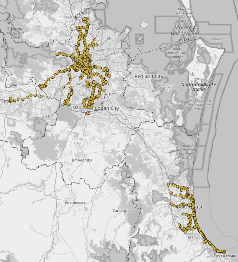
This revealed that SEQ has not one frequent network, but rather several frequent subnetworks. The largest frequent network is the Brisbane one, comprising mostly of BUZ routes but also the frequent core of the QR heavy rail network. The second-largest is on the Gold Coast, based around the G:Link and connected frequent routes. Other items are notable, such as the 600 bus on the southern Sunshine Coast, and the Noosa-Tewantin frequent shuttle.
In total 42 clusters were found for early February 2025. Most of these were otherwise-disconnected pairs and triplets due to combined frequency from several routes between just a couple of stops. One example is in Scarborough (northern Redcliffe). The Dockside & Sydney St cross river ferry represents a standalone pair with a legitimately frequent route.
We can put additional graph connections in when stops are very
physically close in real life, but not directly connected by services or
parent_station. For example, the 740 on the Gold Coast
terminates about 100m down the road from the Cypress Avenue light rail
station. A 200 metre threshold for these extra connections gets us down
to 27 clusters.
Initially I committed GIS crimes here by just taking the hypotenuse of the latitude and longitude, but I have now seen the light and used the haversine formula:
CREATE VIEW CloseFrequents AS
SELECT A.stop_id as this_loc, B.stop_id as next_loc,
    2.0 * 6371000.0 * asin(sqrt(
        (   1.0
            - cos(radians(B.stop_lat - A.stop_lat))
            + cos(radians(A.stop_lat))
            * cos(radians(B.stop_lat))
            * (1.0 - cos(radians(B.stop_lon - A.stop_lon)))
        ) / 2.0
    )) as haver_m
FROM EffectiveDaytimeStopFrequencies A, EffectiveDaytimeStopFrequencies B
WHERE A.stop_id <> B.stop_id
    and haver_m <= 200.0
;

-- select * from EffectiveDaytimeFrequencies where stop_id = 'place_cypsta';
-- select * from CloseFrequents where this_loc = 'place_cypsta';| this_loc | next_loc | min(ratio) |
|---|---|---|
| place_cypsta | place_cavsta | 1.47 |
| place_cypsta | place_spnstn | 1.5 |
| this_loc | next_loc | haver_m |
|---|---|---|
| place_cypsta | 300539 | 157.478940094637 |
| place_cypsta | 300540 | 188.048300729033 |
| place_cypsta | 319488 | 102.387779140933 |
While not shown in the tables above, the vast bulk of connections made here are actually just inbound/outbound bus stop pairs — after all, the bus usually has to stop on both sides of the road! Before adding these connections, radial routes tended to form big petal-shaped loops in the GraphViz visualisation; now they form a ladder.
As it turns out, with that 200m threshold the median and average distances between these paired stops are just over 100m, although with a 200m threshold it’s plausible that some of the next stops along are sneaking in. To pursue this analysis further would mean excluding pairs of stops which have the same route going the same direction. But that’s not what we’re looking to explore today.
Here’s some SQLite CLI commands to get the GraphViz output.
.headers off
.mode list

.once node_pos.gv
select format('%s [pos="%f,%f"];', stop_id, stop_lon, stop_lat) from EffectiveDaytimeStopFrequencies;

.once node_link.gv
select format('%s -- %s;', this_loc, next_loc)
    from (
        select this_loc, next_loc
            from EffectiveDaytimeFrequencies
        union
        select this_loc, next_loc
            from CloseFrequents
            where this_loc < next_loc
        )
;

.sh echo 'graph frequent_network {' | cat - node_pos.gv node_link.gv > frequent_graph.gv
.sh echo '}' >> frequent_graph.gv
.sh dot -Kneato -s1 -Tpdf frequent_graph.gv > frequent_network.pdf

.headers on
Filtering with GraphViz
The GraphViz tool ccomps will find all the connected
components for us. Slightly frustratingly, we don’t need the positional
hints at this stage, but we can filter them out. We also filter
out all the small clusters (leaving just the big two with 20+
nodes):
ccomps -nxz -X%20- < frequent_graph.gv | grep -v 'pos=' > fg_comps.gv
dot -Kneato -s1 -Tpdf -O < fg_comps.gv
This produces first a .gv file with
subgraph entries, then two visualisation PDFs, for the
Brisbane and Gold Coast clusters.
We can scrape fg_comps.gv into a list of stops again,
then add the positional data back in to map it:
sed -nE -e 's/[[:space:]]*(.+) --.*/\1/p' < fg_comps.gv > tmp_a.txt
sed -nE -e 's/.*-- (.+);.*/\1/p' < fg_comps.gv >> tmp_b.txt
cat tmp_a.txt tmp_b.txt | sort | uniq > stop_id_list.txt
rm tmp_a.txt tmp_b.txt.mode csv
CREATE TABLE FrequentStopIds(stop_id TEXT PRIMARY KEY);
.headers off
.import stop_id_list.txt FrequentStopIds
.headers on
.once frequent_effective_stops_bigclusters.csv
SELECT stop_id, stop_name, stop_lat, stop_lon
FROM Stops JOIN FrequentStopIds USING (stop_id);The Final Result
The below image maps out the two major frequent sub-networks in SEQ, using QGIS.
Bonus: Utility Views
When looking at visual representations, I regularly find myself thinking “hang on, which routes go through here again?”
CREATE VIEW StopRoutes AS
SELECT DISTINCT route_short_name, stop_id, coalesce(nullif(parent_station, ''), stop_id) as combo_id
FROM StopTimes JOIN Trips USING (trip_id) JOIN Routes using (route_id) JOIN Stops using (stop_id);
;

-- select route_short_name from StopRoutes where combo_id = 'place_kgbs'
-- intersect
-- select route_short_name from StopRoutes where combo_id = 'place_sbank';| route_short_name |
|---|
| 111 |
| 222 |
| 66 |
| M2 |
Because StopRoutes is undated, both the 66 and the M2
show up as the GTFS I used straddled the changeover!